**This is from a UC Berkeley course project, so the source code is not publicly viewable. If you are an employer interested in viewing my project code, please contact me privately.**

Assignment 3-1: PathTracer

Helen Yang

Part 1: Ray Generation and Intersection

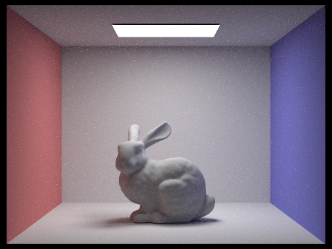
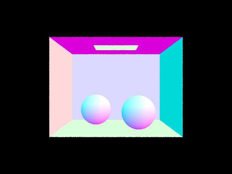
In this part, I first generated random rays through a pixel, sampling random offsets within the pixel's boundaries. Given a \([0,1]\) normalized position in the image plane, rays were generated in the camera plane from the camera position to the point on the virtual camera sensor on the \(Z=-1\) plane, and then converted into world coordinates by multiplying by the camera to world transformation matrix and normalizing.

I implemented intersections between rays and primitives for triangles and spheres. For triangles, I used the Möller–Trumbore intersection algorithm to determine whether a ray would intersect a triangle defined by 3 points. Given a ray defined by its origin point and direction vector \((\vec{O}+ t\vec{D}\)) and a triangle defined by 3 points \((P_0, P_1, P_2)\), this algorithm is an efficient way to determine the \(t\) of intersection and the barycentric coordinates \(b_0\) and \(b_1\) (from which can be determined the third coordinate \(1-b_0-b_1\) defining the position of the intersection within the triangle. For spheres, the \(t\) of intersection can be determined by solving a quadratic equation resulting from substituting the ray formula as \(p\) in the sphere formula \((\vec{p}-\vec{c})^2-R^2=0\) where \(c\) is the center of the sphere and \(R\) is the radius.

If the \(t\) is within our field of view and before any previous intersections (by checking against the ray's t_min and t_max), this means the intersection will occur visible to the camera. If the ray and primitive intersected, I saved the relevant information in an Intersection object, which stored the \(t\) of intersection, normalized surface normal at the intersection point (for triangles, using barycentric coordinates to weight the normals at each of the vertices, and for spheres, the vector from the sphere center to the intersection point), the intersecting primitive, and the material Bidirectional Scattering Distribution Function (BSDF) at the point.

Part 2: Bounding Volume Hierarchy

Bounding Volume Hierarchy (BVH) is a method for organizing primitives to make checking ray-primitive intersection more efficient for rendering. Instead of testing each ray against every single primitive, we only test primitives in bounding boxes that the ray intersects.

The BVH data structure is a tree structure with each node containing a bounding box of its enclosed primitives and non leaf nodes containing references to "left" and "right" child nodes. The bounding box is an axis aligned rectangular prism that contains a primitive (or set of primitives), defined by two 3D points: a min and max corner. The heuristic I used to split "left" and "right" nodes was the average of the centroids of the bounding boxes. I stored the average centroid and compared the number of primitives with centroids on each side of the average centroid when splitting across the x, y, and z axes. I then chose to split along the axis with the most balanced division (minimizing the difference between the number of elements in the "left" and "right" nodes). The BVH was constructed recursively, stopping (creating leaf nodes) when the number of primitives in the node was less than a given amount. There are tradeoffs between different sizes of leaf nodes; having large leaf nodes means that testing ray-primitive intersections of all primitives within the leaf nodes may take longer, but having small leaf nodes means that there will be more bounding box checks needed.

When testing ray intersection, we first check whether the ray intersects the bounding box. If the ray does not intersect the bounding box, none of the primitives inside that bounding box need to be tested for intersection with the ray. If the ray does intersect the bounding box, we can check whether the ray intersects the bounding boxes of the left and right child nodes. This process is repeated recursively until we get to a leaf node, where the ray intersection test is performed against the actual primitives. Because the primitives are not stored in an ordered manner, the first intersection is not necessarily the intersection that is closest to the camera; therefore we must take care to not short circuit the intersection test as soon as an intersection is found. Instead, we keep track of the min and max \(t\) values for the ray to make sure that closer intersections are given priority and intersections are within the camera's field of view.

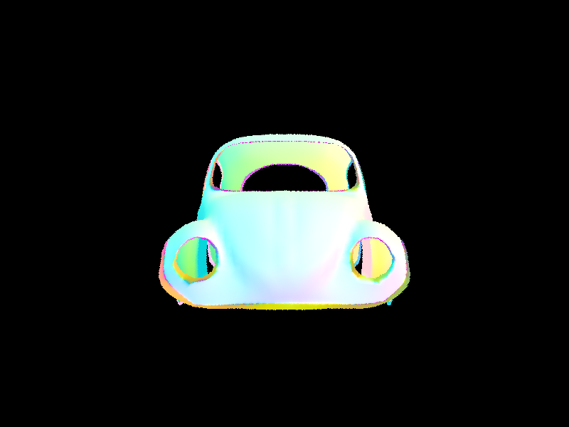
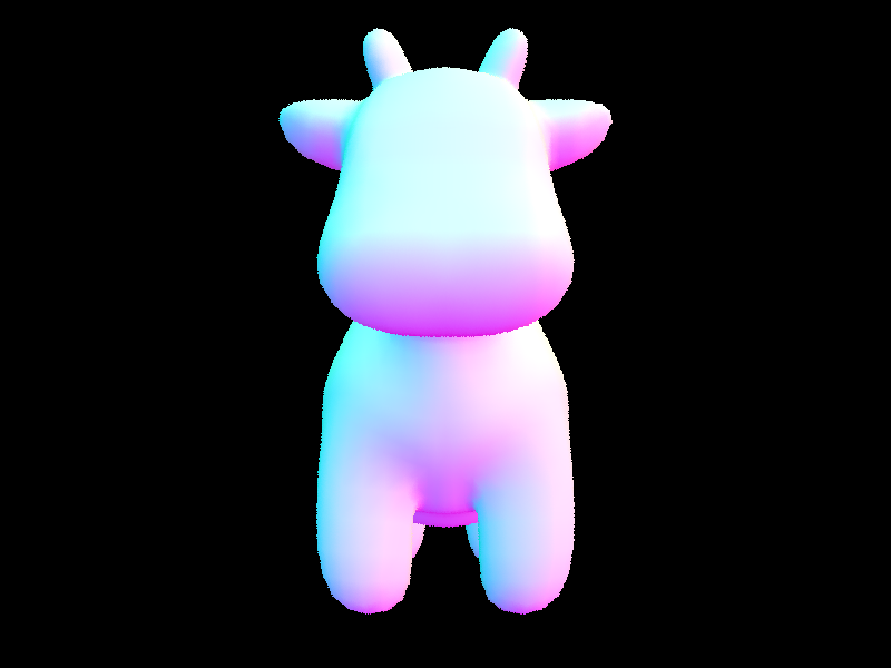
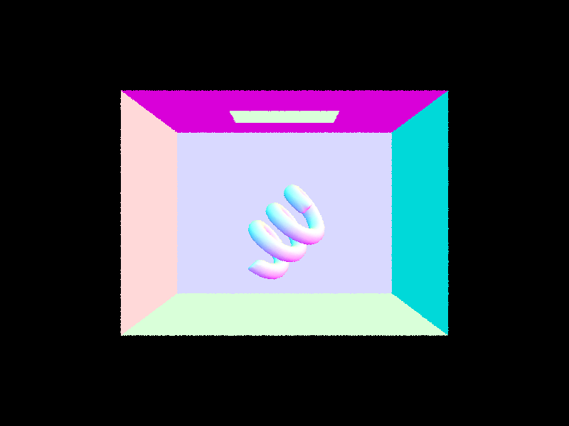
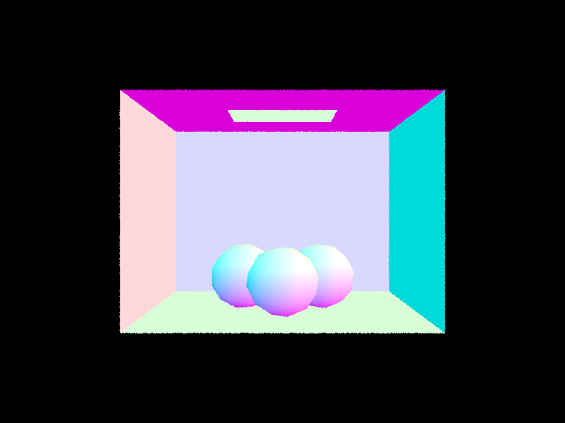
This reduces intersection testing time of a single ray to \(O(\log{n})\) instead of \(O(n)\) where \(n\) is the number of primitives, at the cost of BVH construction and storage and bounding box intersection testing. Using the BVH resulted in very noticeable performance improvements. Our beetle.dae from before, made up of 7558 primitives took 63 seconds to render without a BVH and only 0.10 seconds with the BVH. Similarly, coil.dae with 7884 primitives took 0.12 seconds to render with BVH compared to 62 seconds without. CBgems.dae with 252 primitives took 0.08 seconds and 2.4 seconds to render with and without BVH respectively. On these files, the average number of intersection tests per ray were lower than 5 when using the BVH and sometimes in the hundreds or thousands without the BVH. 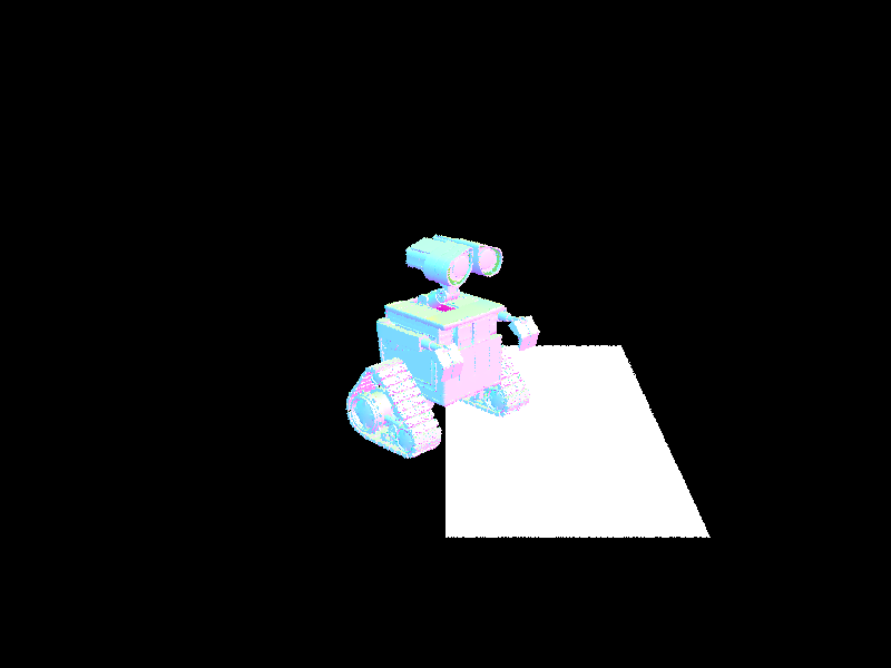Large files like wall-e.dae with 240326 primitives could be rendered in only 0.44 seconds with a BVH while rendering without one was prohibitively slow.