**This is from a UC Berkeley course project, so the source code is not publicly viewable. If you are an employer interested in viewing my project code, please contact me privately.**

CS 184: Computer Graphics and Imaging, Spring 2020

Project 1: Rasterizer

Helen Yang

Overview

In this project, I created a rasterizer that can take vector images (.svg files) and render them into pixel images on a screen and .png files. Some of the viewing options available include supersampling, hierarchical transforms, linear interpolation with barycentric coordinates, and methods of pixel and level sampling for texture maps. Actually implementing the formulas and data structures described in lecture gave me a better understanding of the complexity of rendering even simple shapes. Having the visual feedback and thinking about runtime when trying out different combinations of options helped me solidify my understanding of the tradeoffs between the different methods.

Section I: Rasterization

Part 1: Rasterizing single-color triangles

Rasterizing is the process of taking shape information and converting that into an image by determining which pixels will be colored. In this part, the function for rasterizing triangles takes in a color and 3 \((x,y)\) points which are the vertices of the triangle and colors the pixels within the triangle.

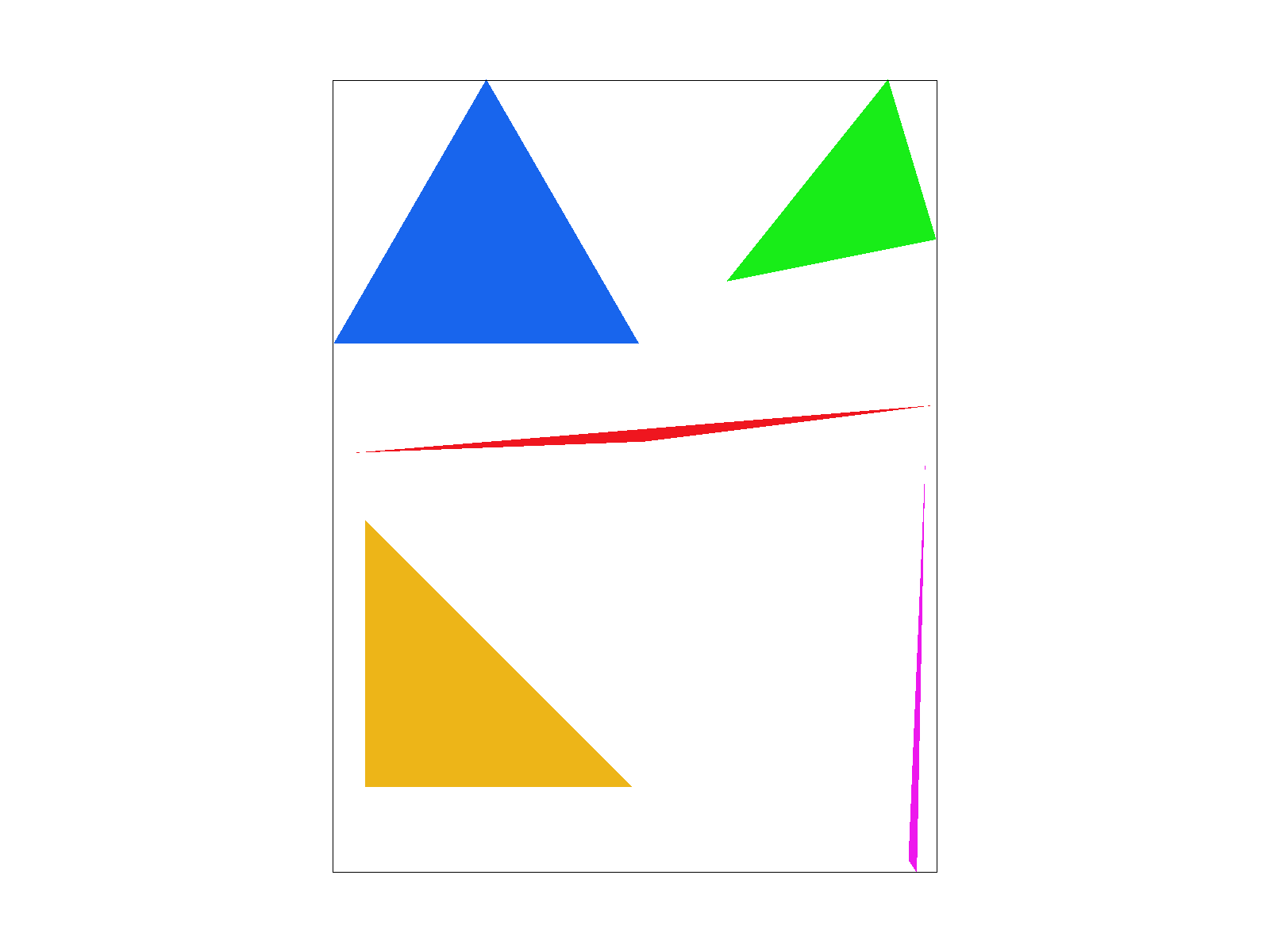
The algorithm I used checks each pixel within the bounding box of the triangle (from the minimum to maximum \(x\) and the minimum to maximum \(y\) of the vertices). For each of these pixels, I determined whether it was within the triangle by testing the pixel (with 0.5 added to each integer coordinate to represent the middle of a square if the pixel coordinates are points on a grid) against the line equations \(L_i(x, y) = -(x-X_i)*(Y_{i+1}-Y_i) + (y-Y_i)*(X_{i+1}-X_i)\) where \((x,y)\) is the point being checked and the coordinates of the vertices are \(X_i, Y_i\). The line equations check which half plane created by a line that the point lies on. Therefore, I needed to do 3 line equation checks for the 3 vertices. Because the formulation assumes an ordering of the vertices, I also needed to do another 3 checks for the opposite winding order. Depending on the value of \(L_i(x, y) = 0\) means the point is on the line, \(> 0\) means the point is inside the edge, and \(< 0\) means the point is outside the edge. The simple edge behavior used was rendering pixels on the line as within the triangle.

Rasterizing triangles: test4.png

There are some obvious aliasing effects ("jaggies"), especially in the red and pink triangles, which will be improved in the next step...

Part 2: Antialiasing triangles

In this part, I implemented grid supersampling to reduce the aliasing effects seen in the previous images. By taking more samples, supersampling is like sampling at a higher resolution and then strategically downsampling. The specific supersampling method used here is grid supersampling, with each pixel having sqrt(sample_rate)samples in each dimension for a total of sample_rate samples that are color averaged into a final single pixel in the framebuffer. This introduced a new buffer to the rendering pipeline containing the Color at each of the supersampled values. Supersampling therefore reduces aliasing artifacts, creating smoother edges at the cost of more required memory for the supersampling buffer.

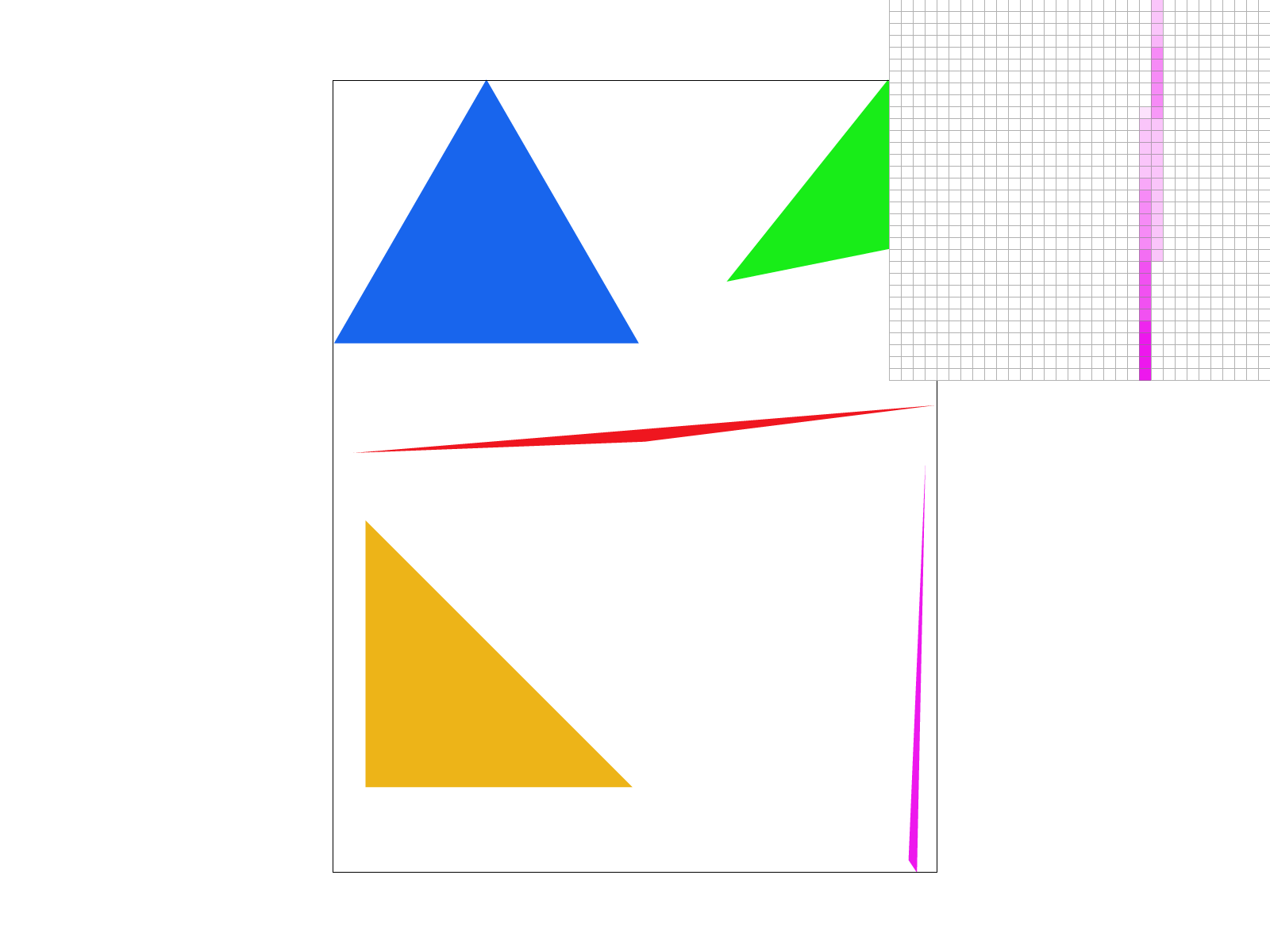
Supersample rate 1 per pixel.	Supersample rate 4 per pixel.
Supersample rate 9 per pixel.	Supersample rate 16 per pixel.

Zooming in with the pixel inspector, we can see the difference on the thin tip of the pink triangle. In the non supersampled image (rate of 1 per pixel), there is a discontinuity, but when supersampled at a rate of 16 per pixel, there is no discontinuity. Without supersampling, when the tip of the triangle becomes very thin, it sometimes does not intersect the middle of the pixel (x+0.5, y+0.5), so there is a discontinuity. When supersampling, at least some of the supersamples within the pixel intersect the middle of the triangle, so they partially weight the color of the triangle so there isn't a completely white discontinuity.

Pixel inspector, not supersampled (1 per pixel).

Pixel inspector, supersampled (16 per pixel).

Part 3: Transforms

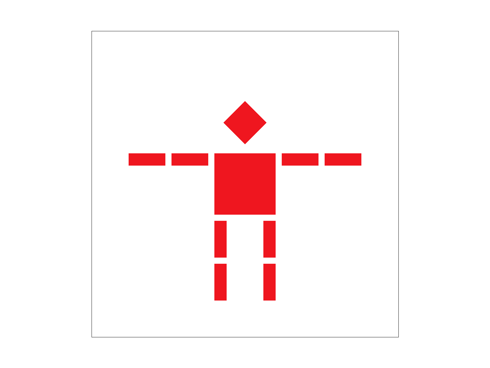
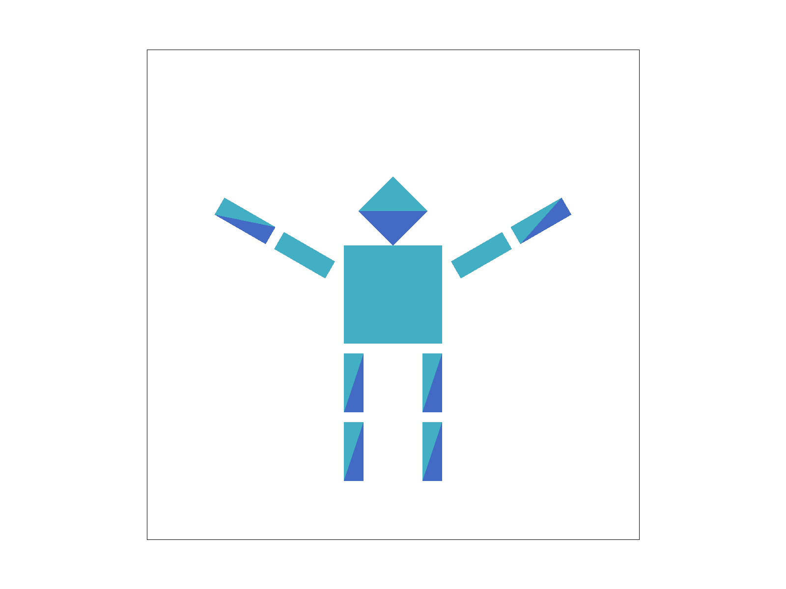
In this section, I implemented 3 basic transforms (translate, scale, and rotate) using transform matrices in homogenous coordinates. To demonstrate the capabilities of these transforms, I created my_robot.svg. I wanted to add more expression to it, so I rotated the arms to be raised, added another color suggesting hands, translated the head down to touch the torso, and flipped (combination of rotation and translation) the left leg so the shadows would be on the same side as the right one.

Original robot.

Robot created with additional hierarchical transformations.

Section II: Sampling

Part 4: Barycentric coordinates

Barycentric coordinates represent a point relative to vertices of a triangle. For a triangle with vertices \((x_n, y_n)\), the barycentric coordinates \((\alpha, \beta\), and \(\gamma\)) of a point \((x, y)\) are related by the equation \((x, y) = \alpha * (x_0, y_0) + \beta * (x_1, y_1) + \gamma * (x_2, y_2)\). In addition, \(\alpha + \beta + \gamma = 1\) so the coordinates can be interpreted as proportions. Conceptually, they can also represent a proportion of area of the triangle created from 2 vertices and the point to the total area of the triangle. If at least one barycentric coordinate is negative, the point is outside of the triangle.

Because barycentric coordinates represent how close a point is to each of the 3 vertices, they are useful to smoothly interpolate between values at each of the vertices, in this case colors. The left image below shows how barycentric coordinates can be used to interpolate between the red, green, and blue vertices. The color at point \(V\) is the color at each of the vertices, weighted by the barycentric coordinates: \(Color(V) = \alpha * Red + \beta * Green + \gamma * Blue\)

A demonstration of how linear interpolation can be used for interpolating between colors .

Color wheel created with barycentric coordinates for interpolating colors.

Part 5: "Pixel sampling" for texture mapping

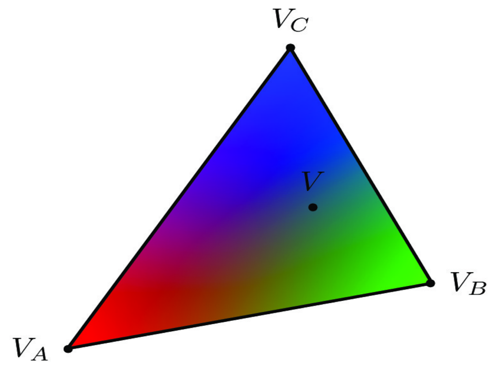
Instead of just interpolating colors given at different vertices, we now have a texture map that tells us what color values should be used. But since the dimensions of the texture map and image don't necessarily match, this is another sampling problem as we need to sample the texture map at the corresponding location for each pixel in the image.

Because we are given the corresponding \((u, v)\) texture coordinates for each of the vertices of the triangle in the image, I used barycentric coordinates to interpolate the texture coordinates for each point within the triangle. The texture coordinates range from 0 to 1, so I multiplied them by the width and height of the texture map to get the actual sample coordinates. In the nearest sampling method, I simply rounded to the nearest sample.

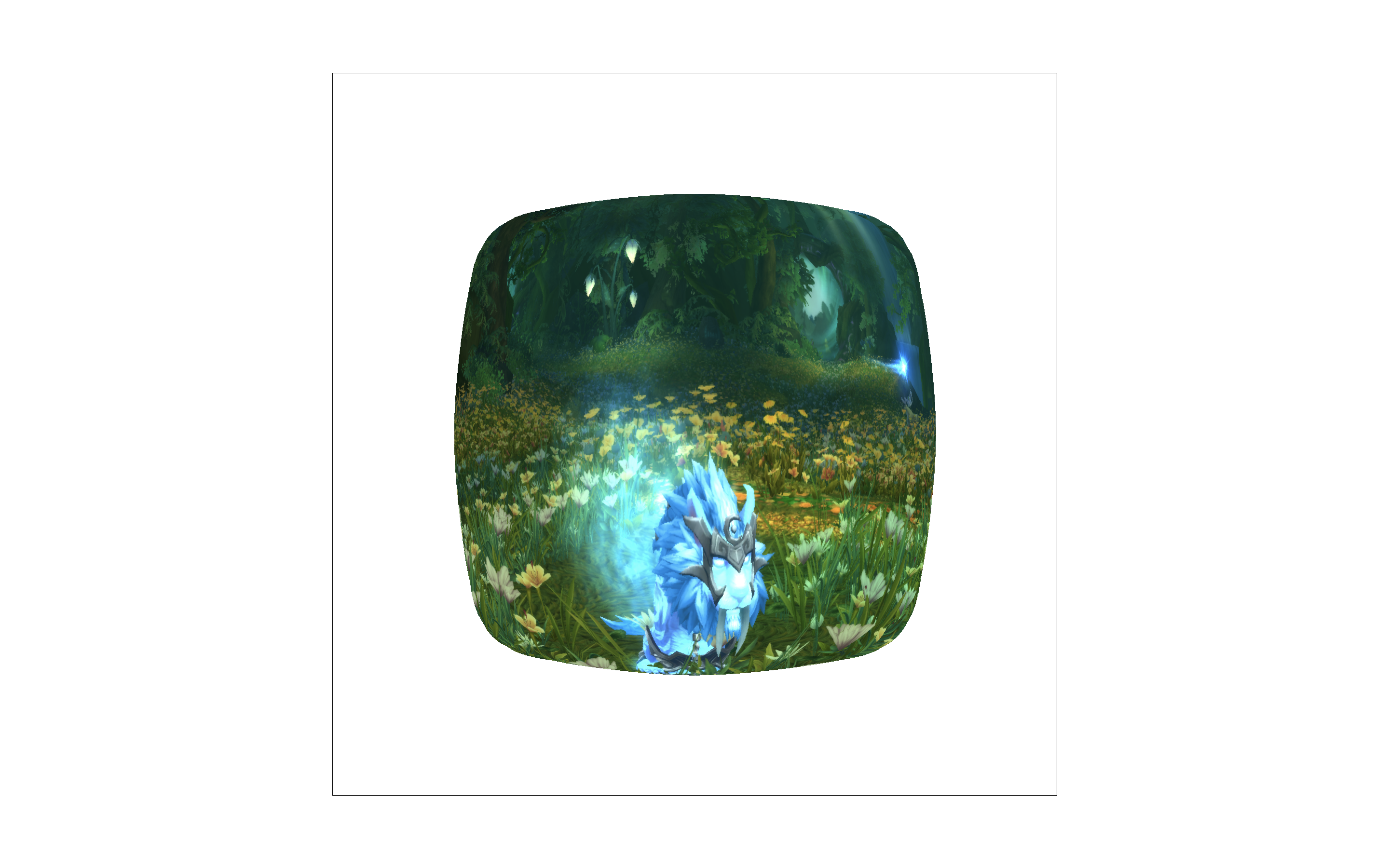
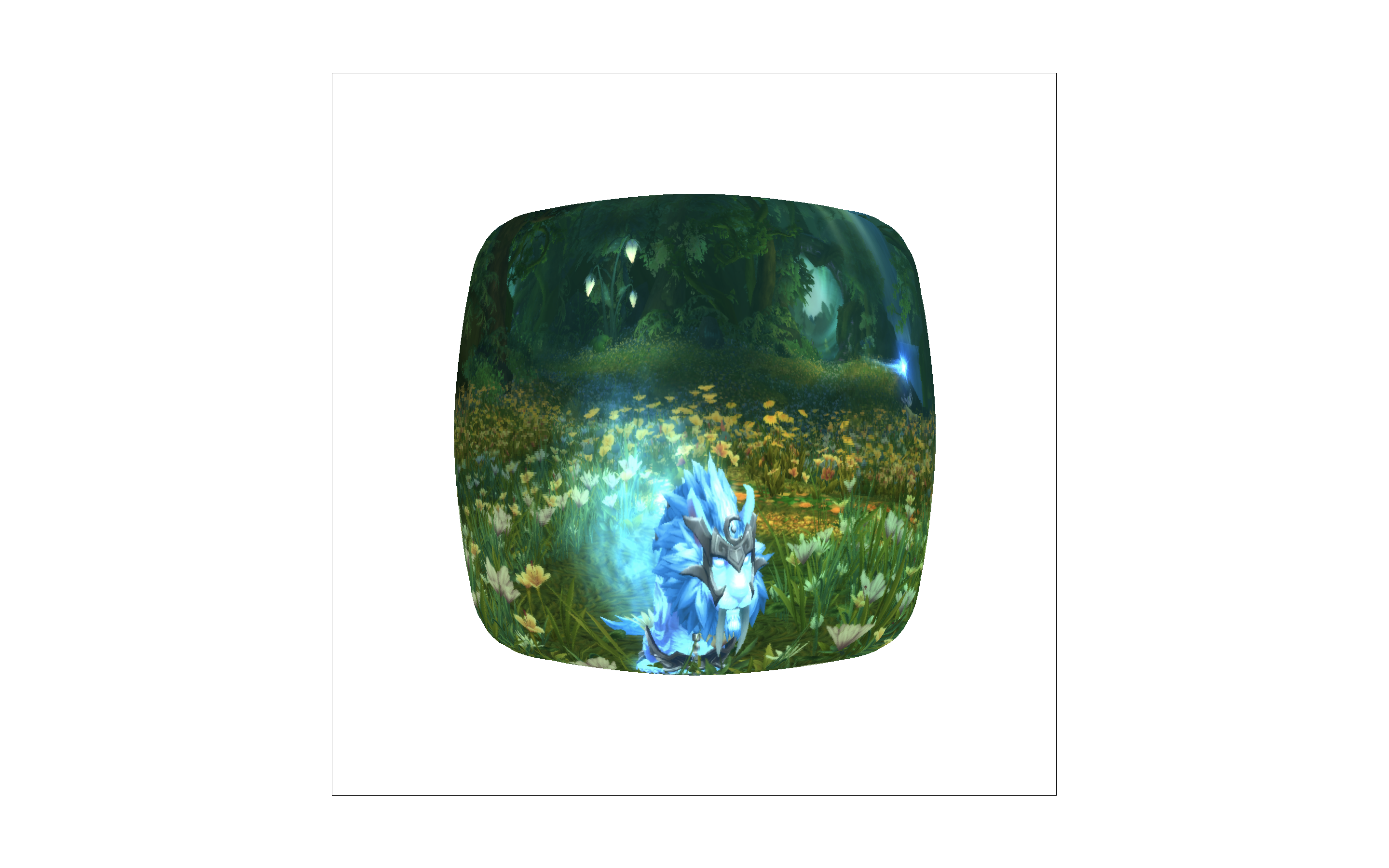
The bilinear interpolation method, takes into account the value of the 4 nearest texels by performing 3 linear interpolations (2 in x and 1 in y) and weighting each of their color values accordingly. There is a larger difference between the two sampling methods in levels with more detail, which often corresponds to higher frequencies.

No supersampling with nearest pixel sampling.	No supersampling with bilinear interpolation.
16 pixels supersampling with nearest pixel sampling.	16 pixels supersampling with bilinear interpolation.

Part 6: "Level sampling" with mipmaps for texture mapping

Mipmaps are series of texture maps of lower and lower resolution. When sampling the color from a texture to render at a specific pixel, the mipmap level sampled depends on the position of the sample. Level sampling imitates how humans view the world; we perceive further away objects at with less detail than closer objects. Level sampling can reduce rendering times and aliasing effects. By sampling at lower resolution, which could be considered a low pass blur filter, aliasing can be reduced. Mipmaps can also help with taking advantage of spatial and temporal locality for memory accesses; in lower resolutions, samples will often be taken sequentially from closer parts of the lower resolution texture map while in the original or higher resolution maps, the sample accesses would be relatively further away from each other. The space complexity tradeoff of using mipmaps is that storage of a mipmap (original texture plus its lower resolution versions) takes up 4/3 the amount of space as storing the original texture alone.

When combined with the pixel sampling options described in the previous section, there are 6 combinations of options. Level zero simply always samples from the highest resolution, or zeroth level mipmap. Nearest sampling uses the level determination formula and rounds the level to the nearest integer. Bilinear filtering, like bilinear pixel interpolation, takes a weighted average of the texture values in the two nearest (using the floor and ceiling operators) integer levels.

Similar to with pixel sampling, bilinear filtering gives a smoother transition between levels at the costs of more samples taken. Level zero sampling tends to look better when the image is more zoomed in because it is closer to the original resolution. But when the image is more zoomed out, you can nearest and bilinear sampling may look better. In the examples below, the difference between the methods is more obvious on the sides and high frequency parts of the image.

Level zero with nearest pixel sampling.	Level zero with bilinear interpolation.
Nearest level with nearest pixel sampling.	Nearest level with bilinear interpolation.
Bilinear level with nearest pixel sampling.	Bilinear level with bilinear interpolation (also known as trilinear texture filtering).